 [1] "blinded_subject_id"    "id_int"                "cohort"
 [4] "age"                   "impact_tmb_score"      "cpb_drug"
 [7] "ecog"                  "best_overall_response" "tt_pfs_d"
[10] "pfs_event"             "tt_os_d"               "event_os"
[13] "TMPT"                  "WMS_SGPID"             "SAMPID"
[16] "total"                 "samp_id"               "identifier.y"
[19] "Shannon"               "tx"                    "age10"
[22] "med_buty"              "fouraminobutyrate"     "gluatarate"
[25] "lysine" "pyruvate" "log_acoa"  Figure 2 - Butyrate Production Capacity from ACoA Pathway and ICB outcome
Here are the column names of the data we are plotting:
fouraminobutyrate, glutarate, lysine and pyruvate represent different parts of the butyrate synthesis pathway.
Panel A
Survival in Mixed Solid Tumor Cohort (n = 147) by ACoA pathway gene abundance in stool above/below the median.
First for overall survival (OS):
# cut the distribution of pyruvate into above/below median:
acoa_df <- acoa_df %>%
  mutate(med_p = cut(pyruvate, quantile(pyruvate, probs=seq(0,1,0.5)), c("Below Median", "Above Median"))) %>% #ifelse(pyruvate > median(pyruvate, na.rm = T), "Above Median", "Below Median")) %>%
  mutate(tt_os_months = tt_os_d/30.44) %>%
  mutate(tt_pfs_months = tt_pfs_d/30.44) %>%
  arrange(med_p)

fit<- survfit(Surv(tt_os_months, event_os) ~ med_p, data = acoa_df)
names(fit$strata) <- gsub("med_p=", "", names(fit$strata))
p <- ggsurvplot(fit,  size = 1,  # change line size
           linetype = "solid", # use solid line
           break.time.by = 12, # break time axis by 12 months
           palette = c("aquamarine4", "coral4"), # custom color palette
           conf.int = TRUE, # Add confidence interval
           pval = TRUE, # Add p-value,
           legend.title="",
           risk.table = TRUE, risk.table.y.text.col = TRUE,
           ylab = "Survival %",
           xlab = "Time (Months)",
           xlim = c(0,48)
           )
print(p)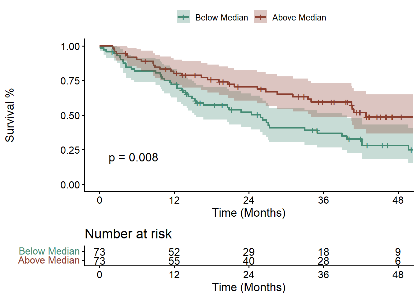
Then looking at Progression Free Survival (PFS) instead of OS:
fit<- survfit(Surv(tt_pfs_months, pfs_event) ~ med_p, data = acoa_df)
names(fit$strata) <- gsub("med_p=", "", names(fit$strata))
p <- ggsurvplot(fit,  size = 1,  # change line size
           linetype = "solid", # use solid line
           break.time.by = 12, # break time axis by 12 months
           palette = c("aquamarine4", "coral4"), # custom color palette
           conf.int = TRUE, # Add confidence interval
           pval = TRUE, # Add p-value,
           legend.title="",
           risk.table = TRUE, risk.table.y.text.col = TRUE,
           ylab = "Survival %",
           xlab = "Time (Months)",
           xlim = c(0,48)
           )
print(p)
Panel B
Restricted cubic spline for Observational cohort adjusted for age, diagnosis, and performance status identifies increasing hazard of overall mortality associated with below-median (<504 RPKM) ACoA pathway gene abundance among ICB recipients. Ticks along the x-axis reflect individual samples.
model_spline_os <- coxph(Surv(tt_os_d, event_os) ~ rms::rcs(pyruvate,4) + age10 + factor(cohort) + ecog, acoa_df)
ptemp <- termplot(model_spline_os, se=T, plot=F)
buterm <- ptemp$pyruvate
center <- buterm$y[which(buterm$y == median(buterm$y))]
ytemp <- buterm$y + outer(buterm$se, c(0, -1.96, 1.96), '*')
exp_ytemp <- exp(ytemp - center)

spline_data <- data.frame(buty = buterm$x, Estimate = exp_ytemp[,1],
                          Lower = exp_ytemp[,2], Upper = exp_ytemp[,3])

ggplot(spline_data, aes(x = buty)) +
  geom_ribbon(aes(ymin = Lower, ymax = Upper), fill = "grey80", alpha = 0.5) +
  geom_line(aes(y = Estimate), color = "blue") +
  geom_rug(sides = "b") +  # Add rug plot at the bottom ('b') of the plot
  scale_y_log10() +  # Log scale for y-axis
  labs(x = "Pyruvate-pathway genes present", y = "Hazard ratio") +
  theme_minimal()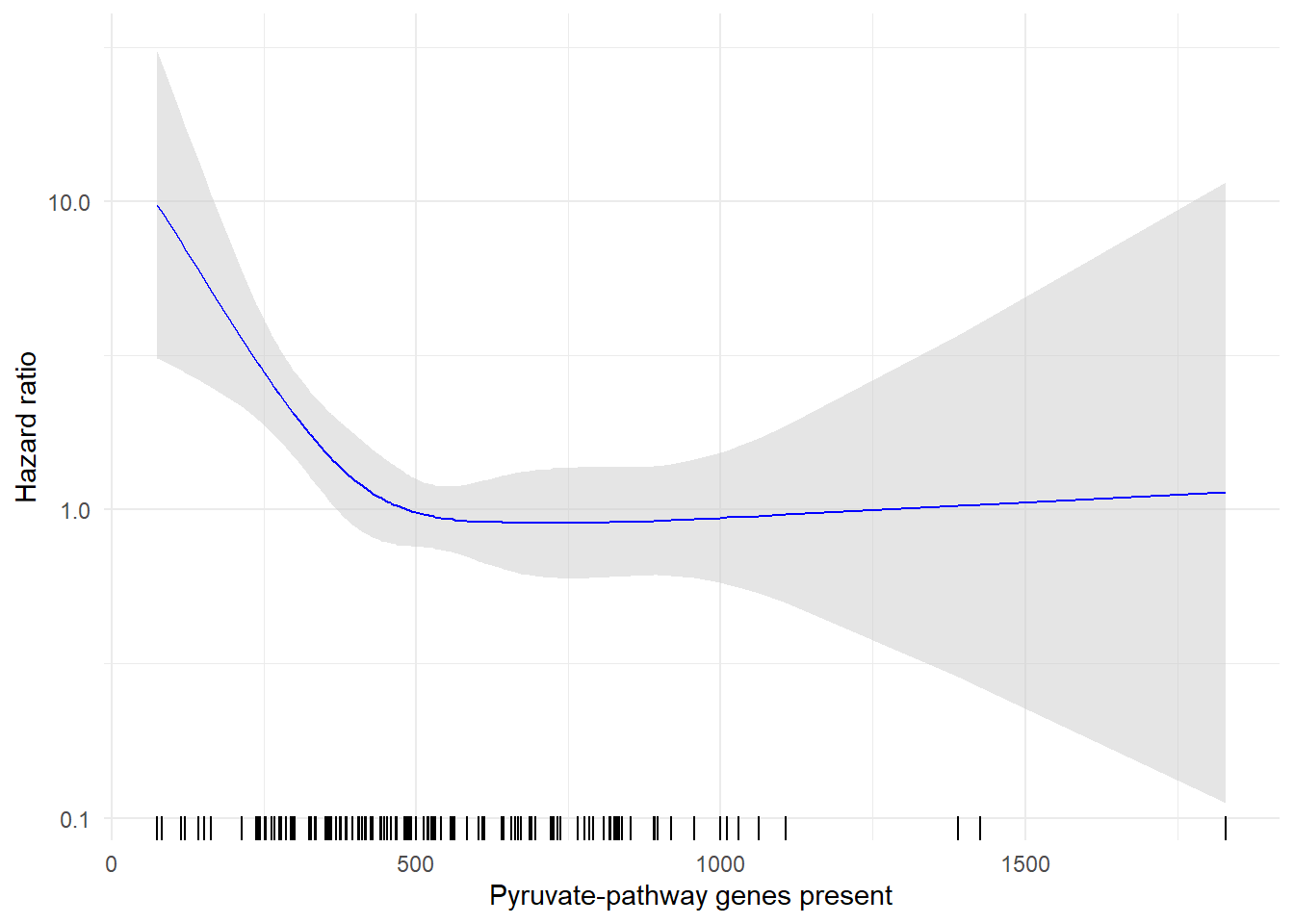
We will now plot some microbiome data, using a phyloseq object that contains our sequencing data. This object contains a list of the taxonomy of organisms identified, the abundance in each sample, and any associated sample specific metadata in one object.
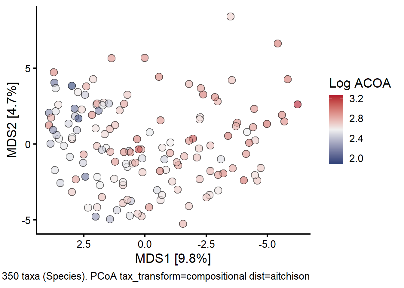
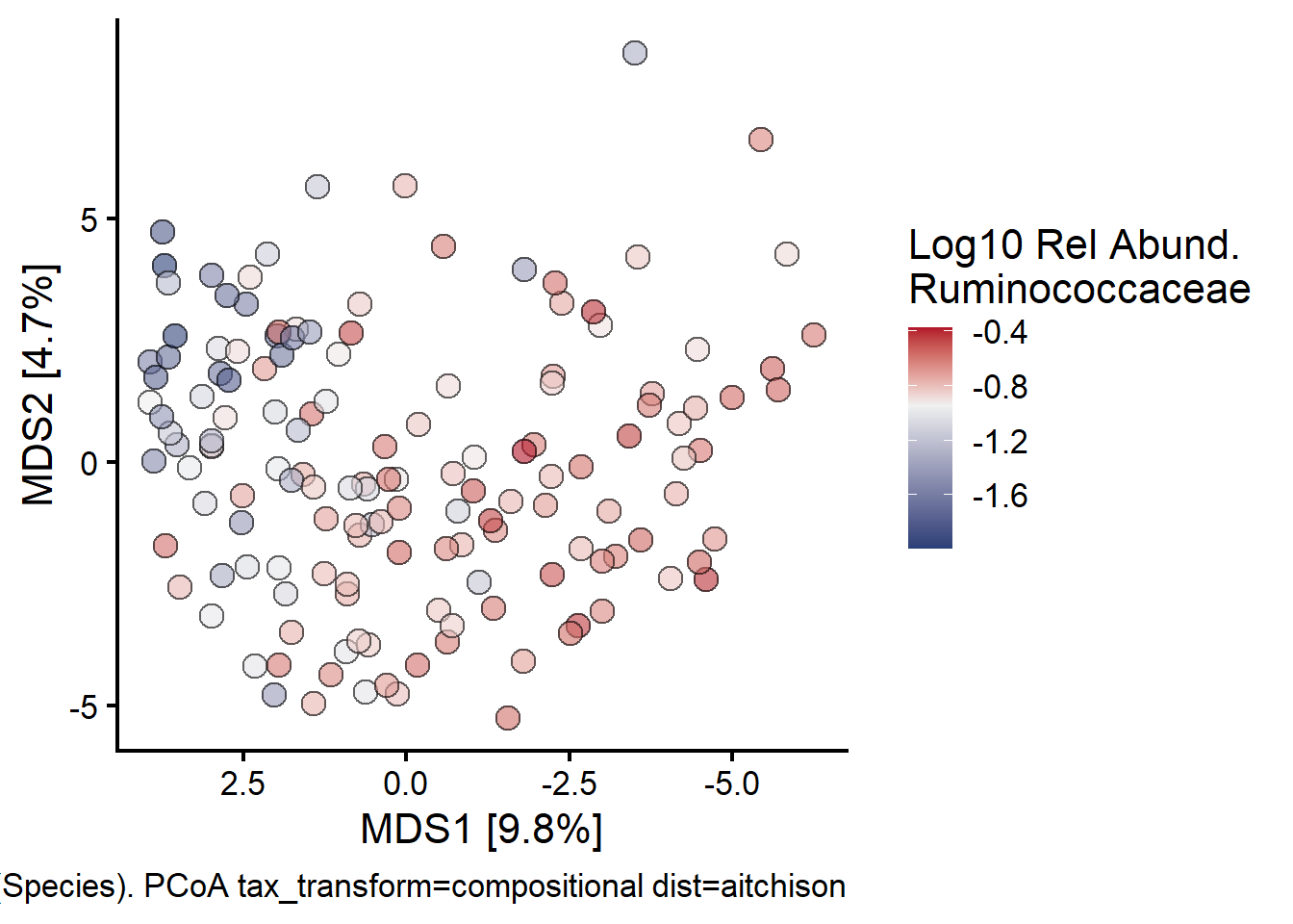
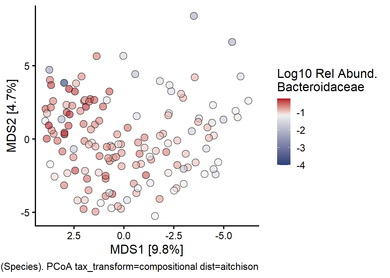
Principal components analysis (PCA) of Observational cohort sample (n = 147, 1 per patient) taxonomic abundance grouped at the family level shows increasing ACoA-pathway gene abundance from left to right along the first principal component (x-axis). Each point represents a single fecal sample. PCA loading vectors (arrows) identify increasing Ruminococcaceae and Lachnospiraceae abundance in the direction corresponding to increased ACoA-pathway gene abundance, versus greater Bacteroidales abundance (grouped at the order level) in the direction of decreased ACoA-pathway gene presence.
Panel C
First looking at how log ACOA distribution looks superimposed over the PCOA of Stool Samples:
ps %>%
  ps_filter(SAMPID %in% acoa_df$SAMPID) %>%
  tax_fix() %>%
  tax_transform(trans = "compositional", rank = "Species") %>%
  dist_calc("aitchison") %>%
  ord_calc("PCoA") %>%
  ord_plot(fill = "log_acoa", size = 4, shape=21, alpha=0.6,
           plot_taxa = c(1:5)) +
  scale_fill_gradientn(colours=c("#2b3f76", "#f0f0f0", "#b2182b"), values=c(0, 0.5, 1)) +
  theme_classic(base_size = 16) +
  scale_x_reverse() +
  labs(
    fill = "Log ACOA"
  )
Next looking at Ruminococcaeceae:
rum_ps <- ps
sample_data(rum_ps)$log_rum = log10(as.numeric(sample_data(ps)$Ruminococcaceae) + 0.0001)
rum_ps %>%
  ps_filter(SAMPID %in% acoa_df$SAMPID) %>%
  tax_fix() %>%
  tax_transform(trans = "compositional", rank = "Species") %>%
  dist_calc("aitchison") %>%
  ord_calc("PCoA") %>%
  ord_plot(fill = "log_rum", size = 4, shape=21, alpha=0.6,
           plot_taxa = c(1:5)) +
  scale_fill_gradientn(colours=c("#2b3f76", "#f0f0f0", "#b2182b"), values=c(0, 0.65, 1)) +
  theme_classic(base_size = 16) +
  scale_x_reverse() +
  labs(
    fill = "Log10 Rel Abund.\nRuminococcaceae"
  )
Lastly looking at Bacteroidaceae:
bac_ps <- ps
sample_data(bac_ps)$log_bac = log10(as.numeric(sample_data(ps)$Bacteroidaceae) + 0.0001)
bac_ps %>%
  ps_filter(SAMPID %in% acoa_df$SAMPID) %>%
  tax_fix() %>%
  tax_transform(trans = "compositional", rank = "Species") %>%
  dist_calc("aitchison") %>%
  ord_calc("PCoA") %>%
  ord_plot(fill = "log_bac", size = 4, shape=21, alpha=0.6,
           plot_taxa = c(1:5)) +
  scale_fill_gradientn(colours=c("#2b3f76", "#f0f0f0", "#b2182b"), values=c(0, 0.75, 1)) +
  theme_classic(base_size = 16) +
  scale_x_reverse() +
  labs(
    fill = "Log10 Rel Abund.\nBacteroidaceae"
  )
Panel D
ACoA-pathway gene abundance was associated with response to ICB among patients with advanced renal cell cancer receiving ipilimumab plus nivolumab in the External Renal Cancer Cohort (n = 39).
coh_base_ni <- readRDS("../data/coh_butyrate.rds")

#Figure 2D
ggplot(coh_base_ni, aes(x = response, y = pyruvate)) +
  geom_boxplot(width = 0.4, outlier.shape = NA, linewidth = 0.6, color = "black") +
  geom_jitter(aes(fill = response), shape = 21, width = 0.15, size = 5, stroke = 0.3, color = "black", alpha = 0.7) +
  scale_fill_manual(values = c("#999999", "#E69F00")) +
  scale_x_discrete(labels = c("Non-responder", "Responder")) +
  theme_classic(base_size = 16) +
  theme(
    legend.position = "none",
    axis.line = element_line(color = "black", linewidth = 0.5),
    axis.ticks = element_line(color = "black", linewidth = 0.5)
  ) +
  xlab("") +
  ylab("ACoA pathway gene abundance (RPKM)")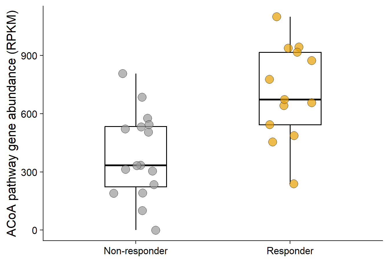
wilcox.test(coh_base_ni$pyruvate ~ coh_base_ni$response)
    Wilcoxon rank sum exact test

data:  coh_base_ni$pyruvate by coh_base_ni$response
W = 36, p-value = 0.002129
alternative hypothesis: true location shift is not equal to 0
group_n <- coh_base_ni %>% count(response)
print(group_n)# A tibble: 2 × 2
response n
<chr> <int>
1 N 16
2 Y 13#adjusted for CMB588
summary(glm(response01 ~ log1p(pyruvate) + cbm588, data = coh_base_ni , family = binomial(link = "logit")))
Call:
glm(formula = response01 ~ log1p(pyruvate) + cbm588, family = binomial(link = "logit"),
data = coh_base_ni)
Coefficients:
Estimate Std. Error z value Pr(>|z|)
(Intercept) -15.157 7.325 -2.069 0.0385 *
log1p(pyruvate) 2.491 1.160 2.148 0.0318 *
cbm588no-CBM -1.439 1.022 -1.407 0.1593
---
Signif. codes: 0 '***' 0.001 '**' 0.01 '*' 0.05 '.' 0.1 ' ' 1
(Dispersion parameter for binomial family taken to be 1)
Null deviance: 39.892 on 28 degrees of freedom
Residual deviance: 26.776 on 26 degrees of freedom
AIC: 32.776
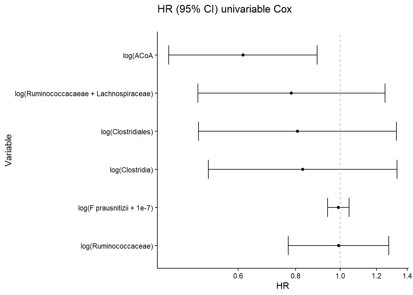
Number of Fisher Scoring iterations: 6Panel E
Univariate Cox regression analyses PFS relationship to ACoA gene abundance in external cohort.
wargo_surv_df <- readRDS("../data/cleaned_data/wargo_pfs_data_for_univariate_model.RDS")


model1_wargo <- coxph(Surv(pfs_d, pfsevent)~log(rum), wargo_surv_df)
model2_wargo <- coxph(Surv(pfs_d, pfsevent)~log(rum_lach), wargo_surv_df)
model3_wargo <- coxph(Surv(pfs_d, pfsevent)~log(clostridiales), wargo_surv_df)
model4_wargo <- coxph(Surv(pfs_d, pfsevent)~log(clostridia), wargo_surv_df)
model5_wargo <- coxph(Surv(pfs_d, pfsevent)~log(eval(faecalibacterium_prausnitzii+1e-7)), wargo_surv_df)
model6_wargo <- coxph(Surv(pfs_d, pfsevent)~log1p(pyruvate), wargo_surv_df)


models <- list(model1_wargo, model2_wargo, model3_wargo, model4_wargo, model5_wargo, model6_wargo)


results_df <- data.frame()


for (i in seq_along(models)) {
  model <- models[[i]]
  summary_model <- summary(model)


  hr <- summary_model$coefficients[, "exp(coef)"]
  lower_ci <- summary_model$conf.int[, "lower .95"]
  upper_ci <- summary_model$conf.int[, "upper .95"]
  pvalue <- summary_model$coefficients[, "Pr(>|z|)"]


  results_df <- rbind(results_df, data.frame(
    Model = paste0("model", i),
    HR = hr,
    Lower_CI = lower_ci,
    Upper_CI = upper_ci,
    pvalue = pvalue
  ))
}

results_df$source = rep("wargo", 6)
results_df$modelname = c("log(Ruminococcaceae)", "log(Ruminococcacaeae + Lachnospiraceae)",
                             "log(Clostridiales)", "log(Clostridia)", "log(F prausnitizii + 1e-7)", "log(ACoA")


ggplot(results_df) +
  geom_point(aes(y=fct_rev(fct_reorder(modelname, HR)), x=HR)) +
  geom_errorbarh(aes(y=fct_rev(fct_reorder(modelname, HR)), xmin=Lower_CI, xmax=Upper_CI), height=0.5)+
  geom_vline(xintercept=1, lty=2, col="gray70") +
  scale_x_continuous(trans="log") +
  theme_classic() +
  labs(title = "HR (95% CI) univariable Cox",
       subtitle ="", y="Variable", x="HR")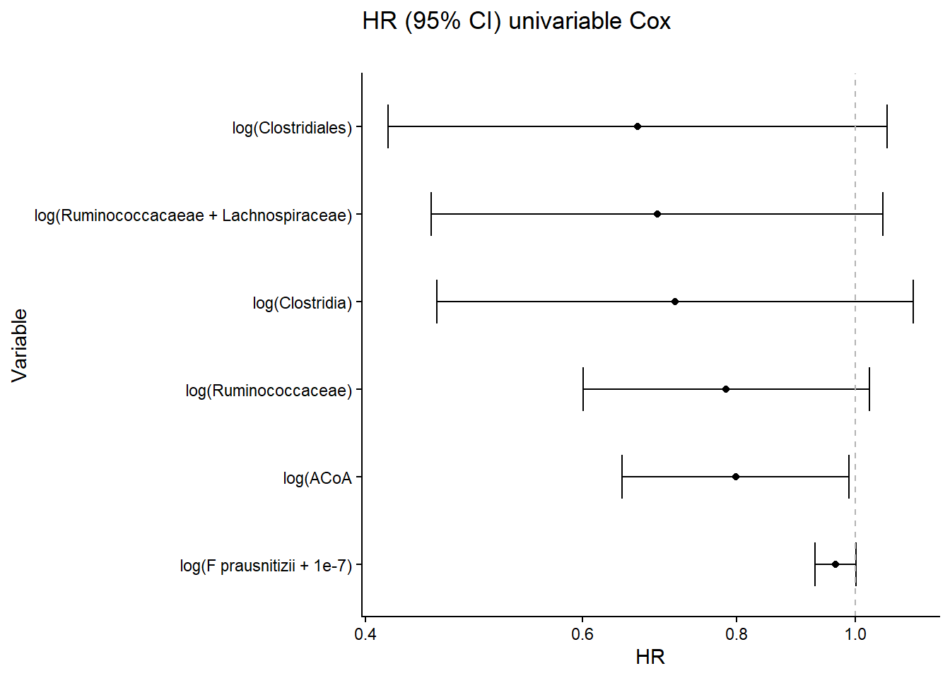
Panel E MSK Data
Univariate Cox regression analyses PFS relationship to ACoA gene abundance in MSK Observational Data.
msk_df <- readRDS("../data/cleaned_data/interal_msk_data_for_univariate_model.RDS")

model1_msk <- coxph(Surv(tt_pfs_d, pfs_event)~log(rum), msk_df)
model2_msk <- coxph(Surv(tt_pfs_d, pfs_event)~log(rum_lach), msk_df)
model3_msk <- coxph(Surv(tt_pfs_d, pfs_event)~log(clostridiales), msk_df)
model4_msk <- coxph(Surv(tt_pfs_d, pfs_event)~log(clostridia), msk_df)
model5_msk <- coxph(Surv(tt_pfs_d, pfs_event)~log(eval(faecalibacterium_prausnitzii+1e-4)), msk_df)
model6_msk <- coxph(Surv(tt_pfs_d, pfs_event)~log1p(pyruvate), msk_df)


models <- list(model1_msk, model2_msk, model3_msk, model4_msk, model5_msk, model6_msk)


results_df <- data.frame()


for (i in seq_along(models)) {
  model <- models[[i]]
  summary_model <- summary(model)


  hr <- summary_model$coefficients[, "exp(coef)"]
  lower_ci <- summary_model$conf.int[, "lower .95"]
  upper_ci <- summary_model$conf.int[, "upper .95"]
  pvalue <- summary_model$coefficients[, "Pr(>|z|)"]


  results_df <- rbind(results_df, data.frame(
    Model = paste0("model", i),
    HR = hr,
    Lower_CI = lower_ci,
    Upper_CI = upper_ci,
    pvalue = pvalue
  ))
}

results_df$source = rep("msk", 6)
results_df$modelname = c("log(Ruminococcaceae)", "log(Ruminococcacaeae + Lachnospiraceae)",
                             "log(Clostridiales)", "log(Clostridia)", "log(F prausnitizii + 1e-7)", "log(ACoA")


ggplot(results_df) +
  geom_point(aes(y=fct_rev(fct_reorder(modelname, HR)), x=HR)) +
  geom_errorbarh(aes(y=fct_rev(fct_reorder(modelname, HR)), xmin=Lower_CI, xmax=Upper_CI), height=0.5)+
  geom_vline(xintercept=1, lty=2, col="gray70") +
  scale_x_continuous(trans="log") +
  theme_classic() +
  labs(title = "HR (95% CI) univariable Cox",
       subtitle ="", y="Variable", x="HR")