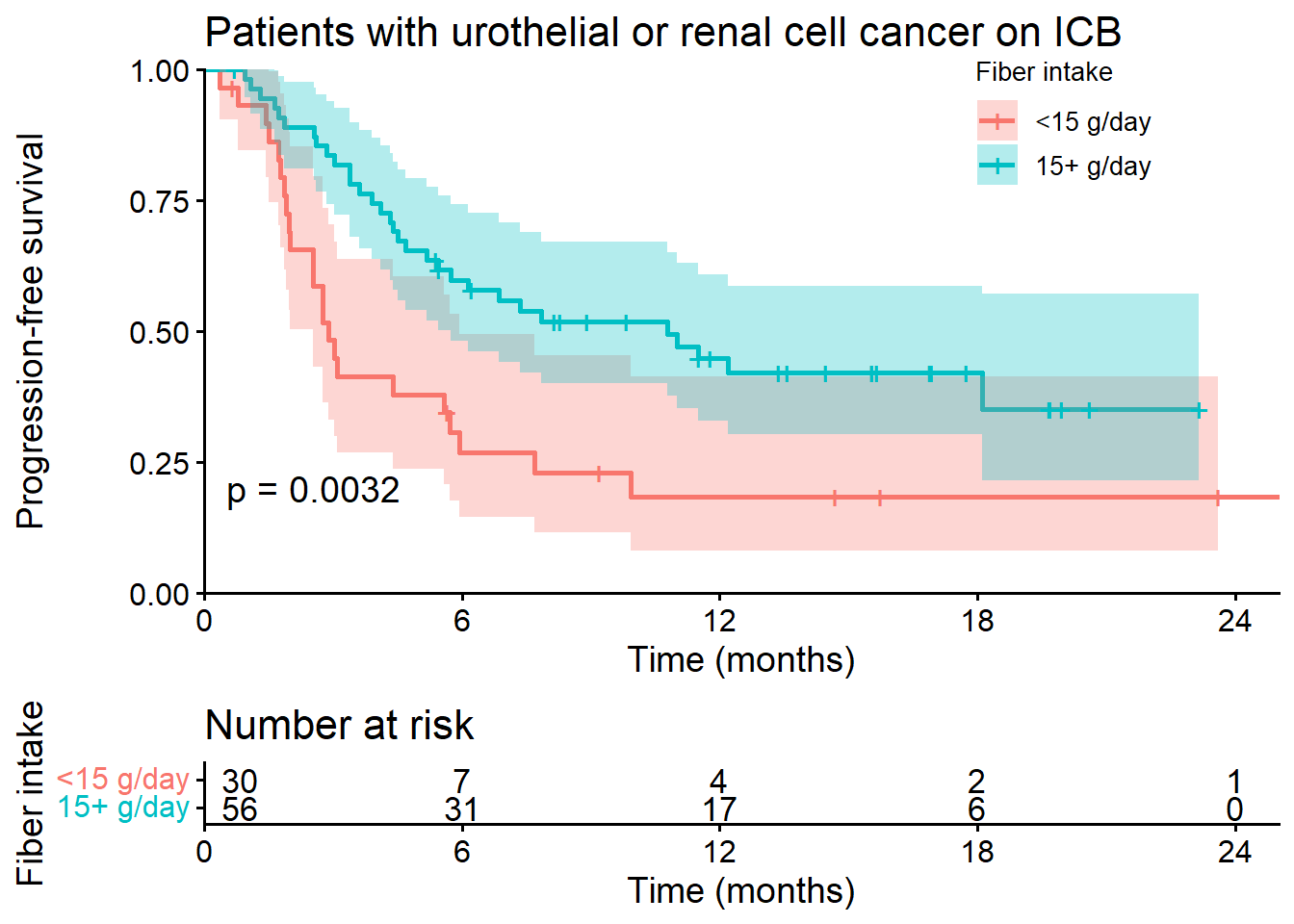
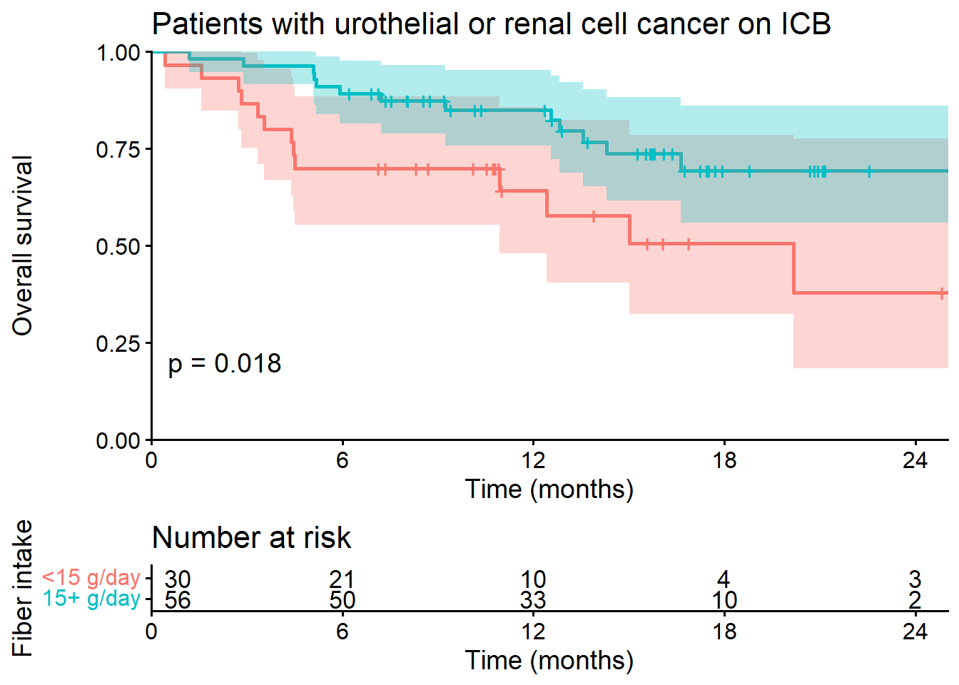
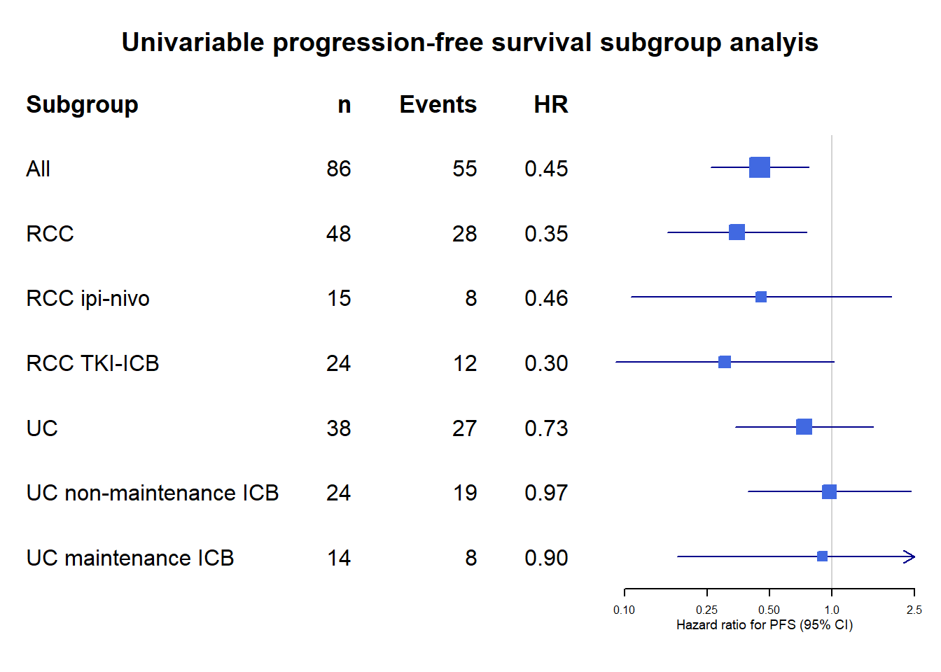
Univariate HRs for PFS among clinically relavant subgroups.
<- coxph (Surv (pfs_mo,pod_status)~ fiber_dichotomized,summary (cox_pfs_all_uv)
Call:
coxph(formula = Surv(pfs_mo, pod_status) ~ fiber_dichotomized,
    data = all_metadata_fiber)

  n= 86, number of events= 55

                      coef exp(coef) se(coef)      z Pr(>|z|)
fiber_dichotomized -0.8011    0.4488   0.2780 -2.882  0.00395 **
---
Signif. codes:  0 '***' 0.001 '**' 0.01 '*' 0.05 '.' 0.1 ' ' 1

                   exp(coef) exp(-coef) lower .95 upper .95
fiber_dichotomized    0.4488      2.228    0.2603    0.7739

Concordance= 0.606  (se = 0.033 )
Likelihood ratio test= 7.82  on 1 df,   p=0.005
Wald test            = 8.31  on 1 df,   p=0.004
Score (logrank) test = 8.74  on 1 df,   p=0.003
<- coxph (Surv (pfs_mo,pod_status)~ fiber_dichotomized,summary (cox_pfs_RC)
Call:
coxph(formula = Surv(pfs_mo, pod_status) ~ fiber_dichotomized,
    data = mRCdataFiber)

  n= 48, number of events= 28

                      coef exp(coef) se(coef)      z Pr(>|z|)
fiber_dichotomized -1.0541    0.3485   0.3945 -2.672  0.00754 **
---
Signif. codes:  0 '***' 0.001 '**' 0.01 '*' 0.05 '.' 0.1 ' ' 1

                   exp(coef) exp(-coef) lower .95 upper .95
fiber_dichotomized    0.3485      2.869    0.1608    0.7551

Concordance= 0.641  (se = 0.046 )
Likelihood ratio test= 6.46  on 1 df,   p=0.01
Wald test            = 7.14  on 1 df,   p=0.008
Score (logrank) test = 7.8  on 1 df,   p=0.005
<- coxph (Surv (pfs_mo,pod_status)~ fiber_dichotomized,summary (cox_pfs_RC_IpiNivo)
Call:
coxph(formula = Surv(pfs_mo, pod_status) ~ fiber_dichotomized,
    data = dataRCIpiNivoFiber)

  n= 15, number of events= 8

                      coef exp(coef) se(coef)      z Pr(>|z|)
fiber_dichotomized -0.7864    0.4555   0.7387 -1.065    0.287

                   exp(coef) exp(-coef) lower .95 upper .95
fiber_dichotomized    0.4555      2.196    0.1071     1.937

Concordance= 0.627  (se = 0.094 )
Likelihood ratio test= 1.04  on 1 df,   p=0.3
Wald test            = 1.13  on 1 df,   p=0.3
Score (logrank) test = 1.19  on 1 df,   p=0.3
<- coxph (Surv (pfs_mo,pod_status)~ fiber_dichotomized,summary (cox_pfs_RC_TKI_IO)
Call:
coxph(formula = Surv(pfs_mo, pod_status) ~ fiber_dichotomized,
    data = dataRCioTKIFiber)

  n= 24, number of events= 12

                      coef exp(coef) se(coef)      z Pr(>|z|)
fiber_dichotomized -1.1926    0.3034   0.6183 -1.929   0.0538 .
---
Signif. codes:  0 '***' 0.001 '**' 0.01 '*' 0.05 '.' 0.1 ' ' 1

                   exp(coef) exp(-coef) lower .95 upper .95
fiber_dichotomized    0.3034      3.295   0.09031      1.02

Concordance= 0.635  (se = 0.073 )
Likelihood ratio test= 3.16  on 1 df,   p=0.08
Wald test            = 3.72  on 1 df,   p=0.05
Score (logrank) test = 4.17  on 1 df,   p=0.04
<- coxph (Surv (pfs_mo,pod_status)~ fiber_dichotomized,summary (cox_pfs_UC)
Call:
coxph(formula = Surv(pfs_mo, pod_status) ~ fiber_dichotomized,
    data = mUCdataFiber)

  n= 38, number of events= 27

                      coef exp(coef) se(coef)      z Pr(>|z|)
fiber_dichotomized -0.3084    0.7346   0.3919 -0.787    0.431

                   exp(coef) exp(-coef) lower .95 upper .95
fiber_dichotomized    0.7346      1.361    0.3408     1.584

Concordance= 0.53  (se = 0.052 )
Likelihood ratio test= 0.61  on 1 df,   p=0.4
Wald test            = 0.62  on 1 df,   p=0.4
Score (logrank) test = 0.62  on 1 df,   p=0.4
<- coxph (Surv (pfs_mo,pod_status)~ fiber_dichotomized,summary (cox_pfs_UC_NOTavelumab)
Call:
coxph(formula = Surv(pfs_mo, pod_status) ~ fiber_dichotomized,
    data = dataUC_NOTavelumabFiber)

  n= 24, number of events= 19

                       coef exp(coef) se(coef)      z Pr(>|z|)
fiber_dichotomized -0.03016   0.97029  0.46269 -0.065    0.948

                   exp(coef) exp(-coef) lower .95 upper .95
fiber_dichotomized    0.9703      1.031    0.3918     2.403

Concordance= 0.473  (se = 0.07 )
Likelihood ratio test= 0  on 1 df,   p=0.9
Wald test            = 0  on 1 df,   p=0.9
Score (logrank) test = 0  on 1 df,   p=0.9
<- coxph (Surv (pfs_mo,pod_status)~ fiber_dichotomized,summary (cox_pfs_UC_avelumab)
Call:
coxph(formula = Surv(pfs_mo, pod_status) ~ fiber_dichotomized,
    data = dataUCavelumabFiber)

  n= 14, number of events= 8

                      coef exp(coef) se(coef)      z Pr(>|z|)
fiber_dichotomized -0.1060    0.8994   0.8239 -0.129    0.898

                   exp(coef) exp(-coef) lower .95 upper .95
fiber_dichotomized    0.8994      1.112    0.1789     4.521

Concordance= 0.527  (se = 0.091 )
Likelihood ratio test= 0.02  on 1 df,   p=0.9
Wald test            = 0.02  on 1 df,   p=0.9
Score (logrank) test = 0.02  on 1 df,   p=0.9
<- tibble:: tibble (mean = c (0.4488 ,0.3485 , 0.4555 , 0.3034 , 0.7346 , 0.97029 , 0.8994 ),lower = c (0.26032 ,0.1608 , 0.1071 , 0.09031 , 0.3408 , 0.3918 , 0.1789 ),upper = c ( 0.7739 ,0.7551 , 1.937 , 1.02 , 1.584 , 2.403 , 4.521 ),study = c ("All" ,"RCC" , "RCC ipi-nivo" , "RCC TKI-ICB" ,"UC" , "UC non-maintenance ICB" , "UC maintenance ICB" ),n = c ("86" ,"48" ,"15" ,"24" ,"38" ,"24" ,"14" ),events = c ("55" ,"28" ,"8" ,"12" ,"27" ,"19" ,"8" ),HR = c ("0.45" ,"0.35" , "0.46" , "0.30" , "0.73" , "0.97" , "0.90" ))|> forestplot (labeltext = c (study, n, events, HR),clip = c (0.09 , 2.5 ),xlog = TRUE ,xlab = "Hazard ratio for PFS (95% CI)" ,xticks = c (0.1 ,0.25 ,0.5 ,1.0 ,2.5 ),title = "Univariable progression-free survival subgroup analyis" ) |> fp_set_style (box = "royalblue" ,line = "darkblue" ,summary = "royalblue" ) |> fp_add_header (study = c ("Subgroup" ),n = c ("n" ),events = c ("Events" ),HR = c ("HR" ))
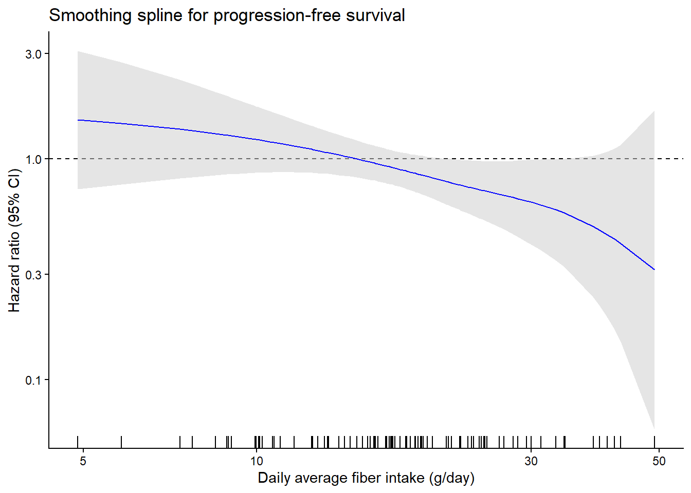
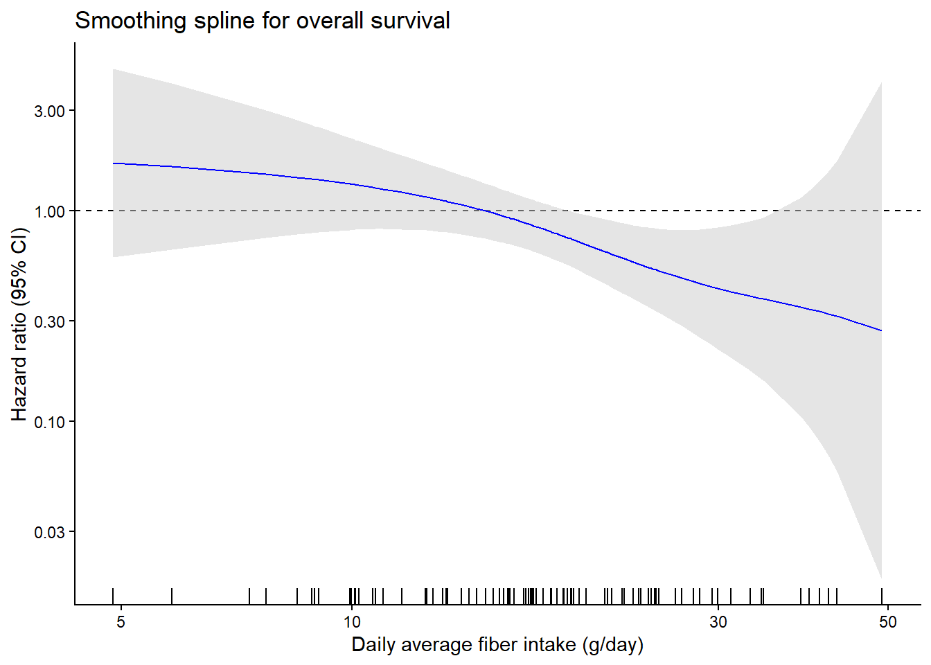
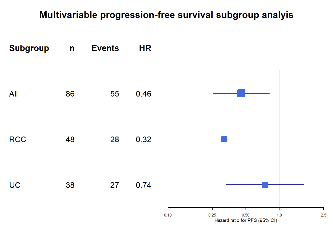
 Figure 1 - Hazard Ratio Analysis of Fiber Intake