get_spline_data <- function(data_df, use_500 = F){
model_spline_os <- coxph(Surv(tt_os_d, event_os)~rcs(pyruvate,4)+age10+strata(cohort)+ecog, data_df)
ptemp <- termplot(model_spline_os, se=T, plot=F)
buterm <- ptemp$pyruvate
if(use_500){
closest_to_500_index <- which.min(abs(buterm$x - 500))
center <- buterm$y[closest_to_500_index]
}else{
center <- buterm$y[which(buterm$y == median(buterm$y))]
}
ytemp <- buterm$y + outer(buterm$se, c(0, -1.96, 1.96), '*')
exp_ytemp <- exp(ytemp - center)
spline_data <- data.frame(buty = buterm$x, Estimate = exp_ytemp[,1],
Lower = exp_ytemp[,2], Upper = exp_ytemp[,3])
return(spline_data)
}
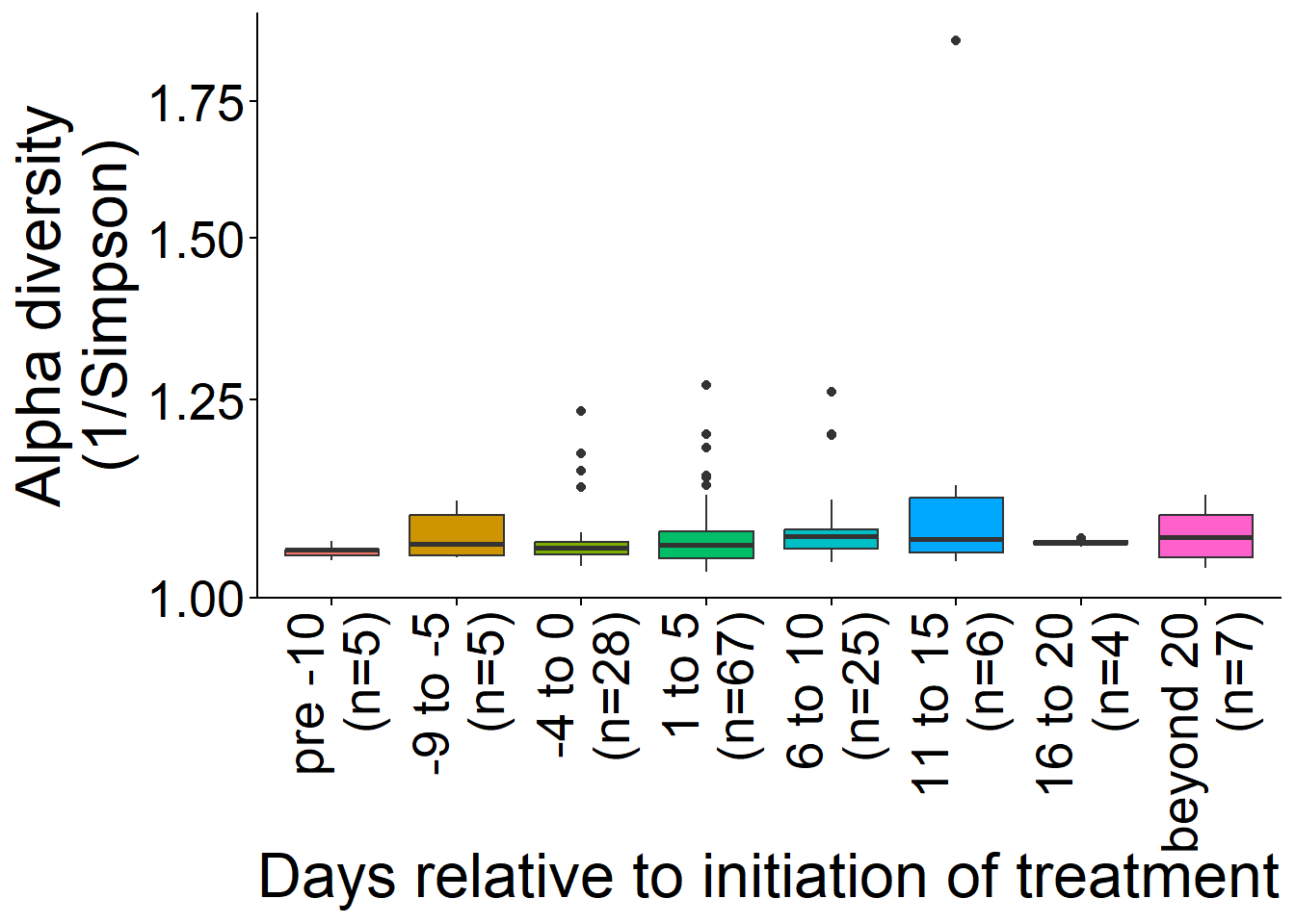
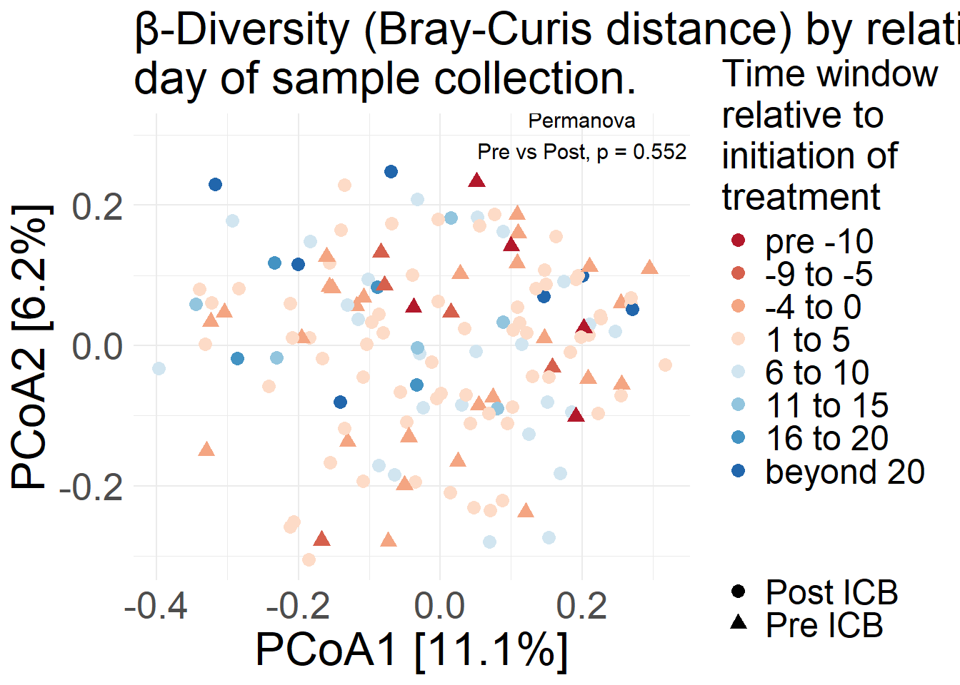
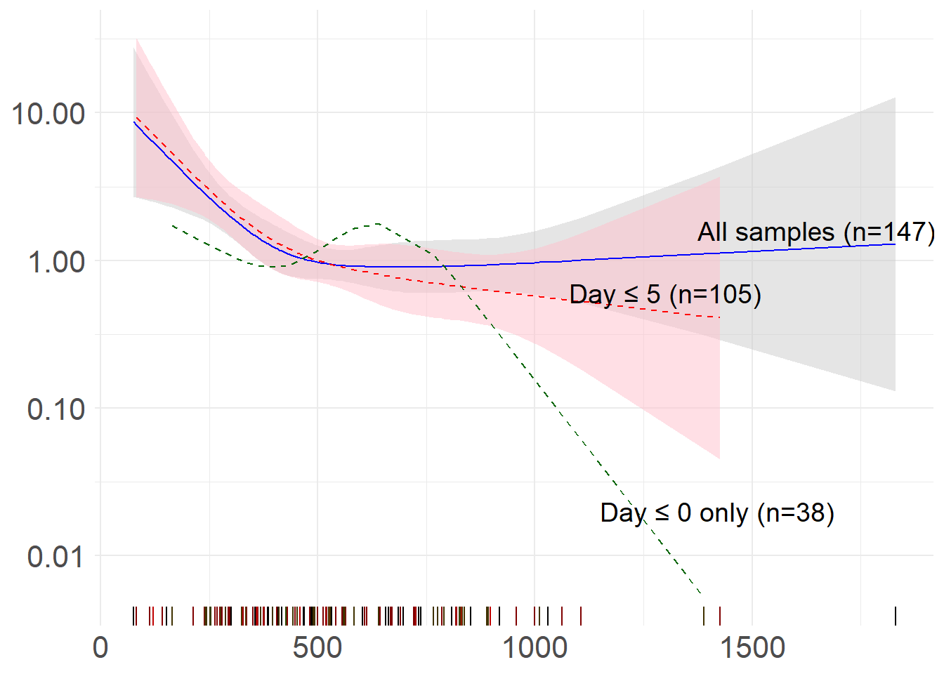
msk_df_pre <- msk_df %>% filter(TMPT <= 0)
msk_df_preplus <- msk_df %>% filter(TMPT <= 5)
spline_data_all <- get_spline_data(msk_df)
spline_data_pre <- get_spline_data(msk_df_pre)
spline_data_preplus <- get_spline_data(msk_df_preplus, use_500 = T)
ggplot()+
geom_ribbon(data=spline_data_all, aes(x=buty, ymin = Lower, ymax = Upper), fill = "grey80", alpha = 0.5) +
geom_ribbon(data=spline_data_preplus, aes(x=buty, ymin = Lower, ymax = Upper), fill = "pink", alpha = 0.5, lty=2) +
#geom_ribbon(data=spline_data_pre, aes(x=buty, ymin = Lower, ymax = Upper), fill = "lightblue", alpha = 0.25) +
geom_line(data=spline_data_all, aes(x=buty, y = Estimate), color = "blue") +
geom_line(data=spline_data_preplus, aes(x=buty, y = Estimate), color = "red", lty=2) +
geom_line(data=spline_data_pre, aes(x=buty, y = Estimate), color = "darkgreen", lty=2.5) +
geom_rug(data=spline_data_all, aes(x=buty), sides = "b") + # Add rug plot at the bottom ('b') of the plot
geom_rug(data=spline_data_preplus, aes(x=buty), sides = "b", color="red", alpha=0.5) + # Add rug plot at the bottom ('b') of the plot
geom_rug(data=spline_data_pre, aes(x=buty), sides = "b", color="darkgreen", alpha=0.5) +
annotate("text", x = 1650, y = 1.6, label = paste0("All samples (n=", nrow(msk_df), ")"), color = "black", size = 5) +
annotate("text", x = 1300, y = .6, label = paste0("Day ≤ 5 (n=", nrow(msk_df_preplus), ")"), color = "black", size = 5) +
annotate("text", x = 1420, y = .02, label = paste0("Day ≤ 0 only (n=", nrow(msk_df_pre), ")"), color = "black", size =5) +
scale_y_log10() + # Log scale for y-axis
labs(
x = "ACoA-pathway genes present",
y = "Hazard ratio",
title = "Sensitivity analysis - day of sample collection relative to start of therapy") +
theme_minimal() +
theme(text = element_text(size=20),
title = element_blank())