 [1] "blinded_subject_id"    "id_int"                "cohort"
 [4] "age"                   "impact_tmb_score"      "cpb_drug"
 [7] "ecog"                  "best_overall_response" "tt_pfs_d"
[10] "pfs_event"             "tt_os_d"               "event_os"
[13] "TMPT"                  "WMS_SGPID"             "SAMPID"
[16] "total"                 "samp_id"               "identifier.y"
[19] "Shannon"               "tx"                    "age10"
[22] "med_buty"              "fouraminobutyrate"     "gluatarate"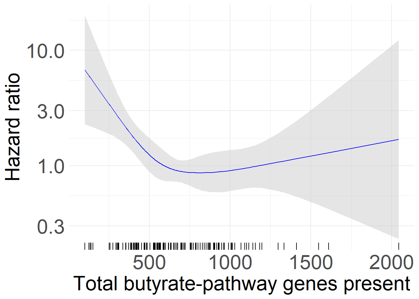
[25] "lysine" "pyruvate" Extended Figure 2 Gene Abundance and Hazard Ration, and Univatiate Analysis of Butyrate Pathway.
Panel A
Hazard Ratio of Overall Survival Evaluated with respect to Butyrate production gene RPKM.
os_butyrate <-  coxph(Surv(tt_os_d, event_os)~rms::rcs(total,4)+age10+factor(cohort)+ecog,, data = acoa_df)
ptemp <- termplot(os_butyrate, se=T, plot=F)
buterm <- ptemp$total
center <- buterm$y[which(buterm$y == median(buterm$y))]
ytemp <- buterm$y + outer(buterm$se, c(0, -1.96, 1.96), '*')
exp_ytemp <- exp(ytemp - center)

spline_data <- data.frame(buty = buterm$x, Estimate = exp_ytemp[,1],
                          Lower = exp_ytemp[,2], Upper = exp_ytemp[,3])

ggplot(spline_data, aes(x = buty)) +
  geom_ribbon(aes(ymin = Lower, ymax = Upper), fill = "grey80", alpha = 0.5) +
  geom_line(aes(y = Estimate), color = "blue") +
  geom_rug(sides = "b") +  # Add rug plot at the bottom ('b') of the plot
  scale_y_log10() +  # Log scale for y-axis
  labs(x = "Total butyrate-pathway genes present", y = "Hazard ratio") +
  theme_minimal() +
 theme(
     axis.text = element_text(size = 24), # Adjust axis labels
     axis.title = element_text(size = 24), # Adjust axis titles
     plot.title = element_text(size = 24),  # Adjust plot title
     legend.text = element_text(size = 18),  # Adjust legend text
     legend.title = element_text(size = 20), # Adjust legend titleMetronidazole
     strip.text.x = element_text(size = 20),
     strip.text.y = element_text(size = 20)
) 
ggsave("svg/extended_figure_2_part_a_HR_tot_butyrate.svg", w = 6.5, h = 4) Panel B
Univariate model of OS as a function of total butyrate genes, and each major sub-pathway in the butyrate production gene pathways.
univ2 <- function(cox, k=1, l=1){
  coef <- exp(coef(cox))
  confint <- exp(confint(cox))
  p <- summary(cox)$coefficients[,5]
  out <- data.frame("HR"=round(coef,4), round(confint,4), "p"=round(p,9))
  q <- nrow(out)
  if(l== -1){out <- out[q,]
  }else{out <- out[k:l,]}
  return(out)

}

forest_os <- rbind(
univ2(coxph(Surv(tt_os_d, event_os)~log(total)+age10+cohort+ecog, acoa_df)),
univ2(coxph(Surv(tt_os_d, event_os)~log(pyruvate)+age10+cohort+ecog, acoa_df)),
univ2(coxph(Surv(tt_os_d, event_os)~log(lysine+0.0000001)+age10+cohort+ecog, acoa_df)),
univ2(coxph(Surv(tt_os_d, event_os)~log(fouraminobutyrate+0.000001)+age10+cohort+ecog, acoa_df)),
univ2(coxph(Surv(tt_os_d, event_os)~log(gluatarate+0.000001)+age10+cohort+ecog, acoa_df)))

forest_os %>%
  rename_with(~ c("HR", "CI_low", "CI_high", "p"), .cols = everything()) %>%
  rownames_to_column("scfa") %>%
  ggplot() +
  geom_vline(xintercept=1, lty=2, size=0.25)+
  geom_point(aes(x=HR, y=fct_reorder(scfa, HR, .desc = T)))+
  geom_linerange(aes(xmin=CI_low, xmax=CI_high, y=fct_reorder(scfa, HR)), size=0.5) +
  scale_x_continuous(transform = "log", breaks=round(exp(seq(-2,1.5,0.5)),1)) +
  theme_classic() +
  coord_cartesian(xlim=exp(c(-2, 0.3))) +
  labs(y = "") +
 theme(
     axis.text = element_text(size = 20), # Adjust axis labels
     axis.title = element_text(size = 20), # Adjust axis titles
     plot.title = element_text(size = 20),  # Adjust plot title
     legend.text = element_text(size = 18),  # Adjust legend text
     legend.title = element_text(size = 18), # Adjust legend titleMetronidazole
     strip.text.x = element_text(size = 18),
     strip.text.y = element_text(size = 18)
 ) +
theme(axis.text.x = element_text(angle = 90, vjust = 0.5, hjust=1))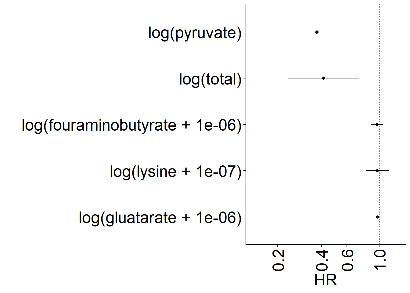
ggsave("svg/extended_figure_2_part_b_forest_plt.svg", w = 6.5, h = 4)