Extended Figure 4 deeper dive into relationship between ACOA pathway abundance and microbiome taxonomy.

Relationship between relative abundance of top families and Acetyl-CoA pathway abundance

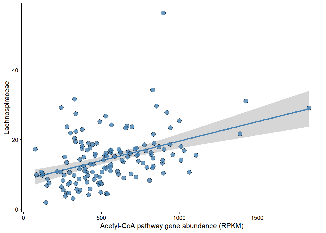
Panel A

Relationship between Rel Abundance of Lachnospiraceae and Acetyle-CoA pathway abundance.

plotting_ps %>%
  filter(grepl("Lachnospiraceae", Family)) %>%
  ggplot() +
  geom_smooth(aes(x=acoa, y=Abundance), method=lm, color="steelblue") +
  geom_point(aes(x=acoa, y=Abundance),
             shape=21, size=3, fill="steelblue", alpha=0.8) +
  theme_classic() + 
  labs(
    x = "Acetyl-CoA pathway gene abundance (RPKM)",
    y = "Lachnospiraceae"
  )

ggsave("svg/extended_figure_4_part_a_Lachnospiraceae.svg", w=5, h = 5)

#|warning: false
#|label: p_value_panel_a
fit <- lm(Abundance ~ acoa, plotting_ps %>%
  filter(grepl("Lachnospiraceae", Family)))
summary(fit)

Call:
lm(formula = Abundance ~ acoa, data = plotting_ps %>% filter(grepl("Lachnospiraceae", 
    Family)))

Residuals:
   Min     1Q Median     3Q    Max 
-9.982 -4.407 -1.105  2.090 37.986 

Coefficients:
            Estimate Std. Error t value Pr(>|t|)    
(Intercept) 8.418826   1.232703   6.830 2.17e-10 ***
acoa        0.011170   0.001998   5.589 1.10e-07 ***
---
Signif. codes:  0 '***' 0.001 '**' 0.01 '*' 0.05 '.' 0.1 ' ' 1

Residual standard error: 6.725 on 145 degrees of freedom
Multiple R-squared:  0.1773,    Adjusted R-squared:  0.1716 
F-statistic: 31.24 on 1 and 145 DF,  p-value: 1.096e-07

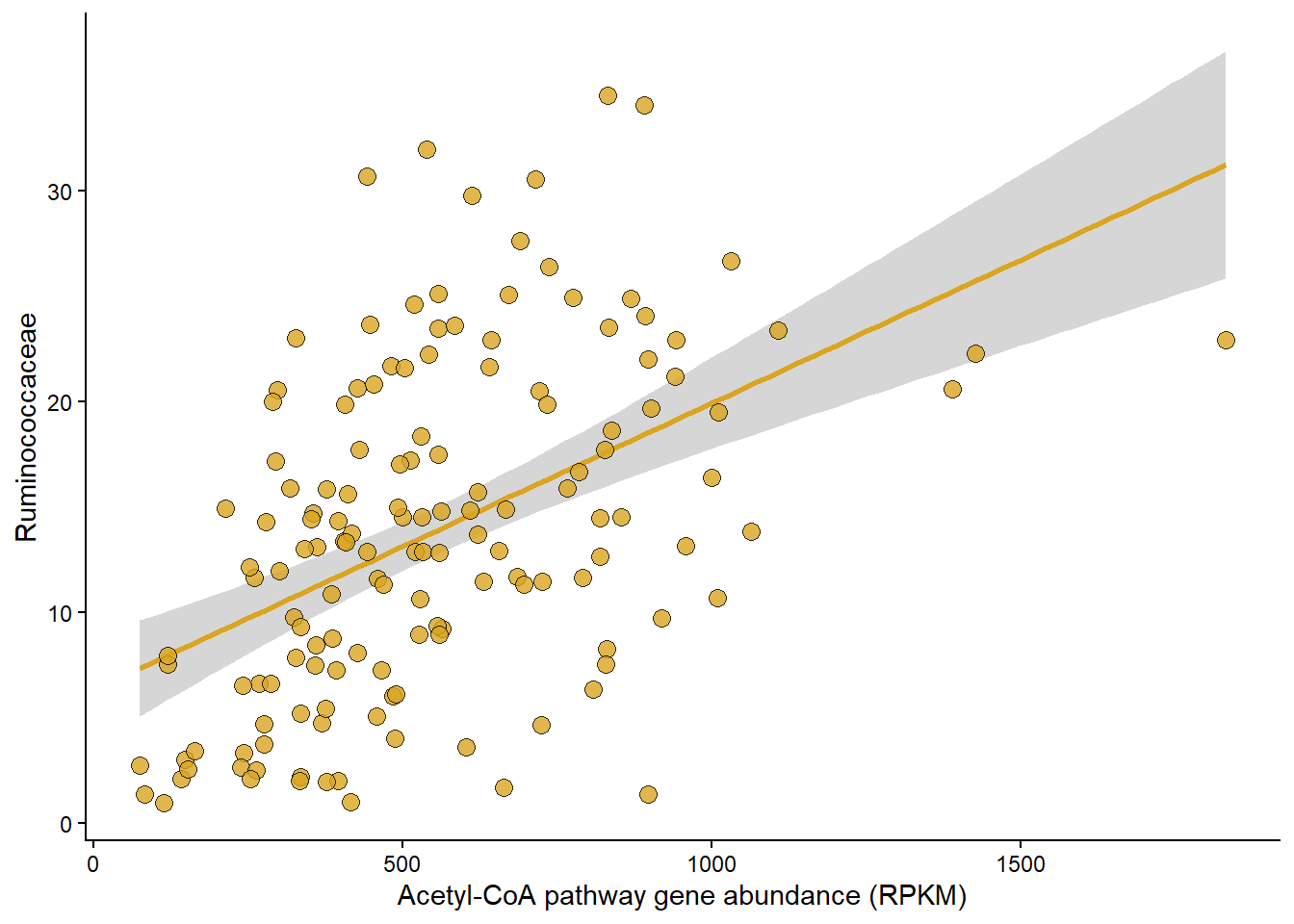
Panel B

Relationship between Rel Abundance of Ruminococcacae and Acetyle-CoA pathway abundance.

plotting_ps %>%
  filter(grepl("Ruminococcaceae", Family)) %>%
  ggplot() +
  geom_smooth(aes(x=acoa, y=Abundance), method=lm, color="goldenrod") +
  geom_point(aes(x=acoa, y=Abundance),
             shape=21, size=3, fill="goldenrod", alpha=0.8) +
  theme_classic() + 
  labs(
    x = "Acetyl-CoA pathway gene abundance (RPKM)",
    y = "Ruminococcaceae"
  )

ggsave("svg/extended_figure_4_part_b_Ruminococcaceae.svg", w=5, h = 5)

#|warning: false
#|label: p_value_panel_b
fit <- lm(Abundance ~ acoa, plotting_ps %>%
  filter(grepl("Ruminococcaceae", Family)))
summary(fit)

Call:
lm(formula = Abundance ~ acoa, data = plotting_ps %>% filter(grepl("Ruminococcaceae", 
    Family)))

Residuals:
     Min       1Q   Median       3Q      Max 
-17.1756  -5.2271  -0.5834   4.2678  18.3653 

Coefficients:
            Estimate Std. Error t value Pr(>|t|)    
(Intercept) 6.310352   1.285751   4.908 2.45e-06 ***
acoa        0.013612   0.002084   6.530 1.04e-09 ***
---
Signif. codes:  0 '***' 0.001 '**' 0.01 '*' 0.05 '.' 0.1 ' ' 1

Residual standard error: 7.014 on 145 degrees of freedom
Multiple R-squared:  0.2272,    Adjusted R-squared:  0.2219 
F-statistic: 42.64 on 1 and 145 DF,  p-value: 1.037e-09

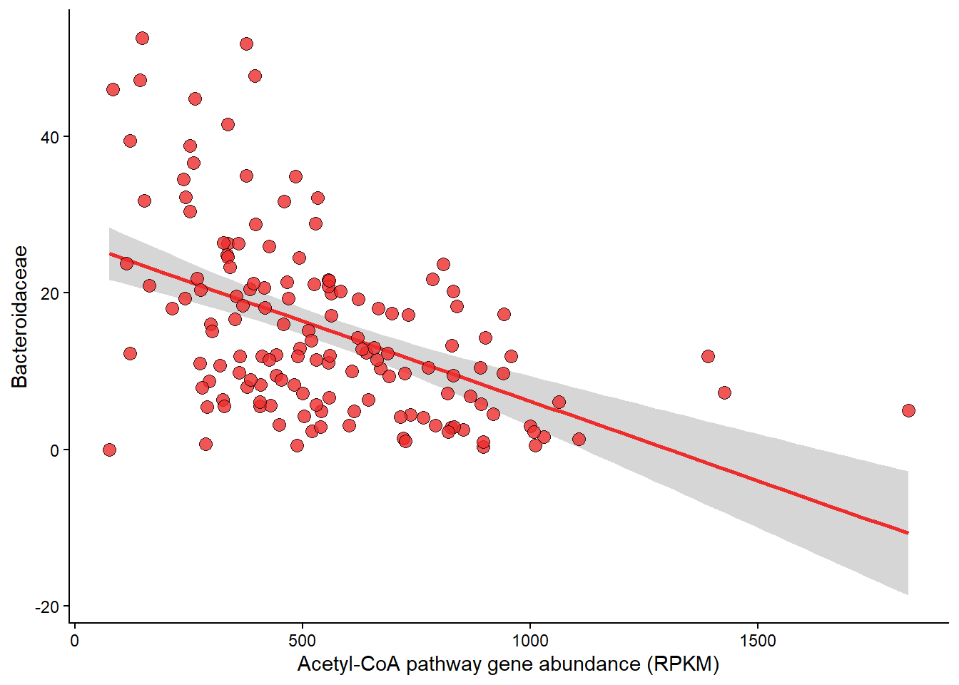
Panel C

Relationship between Rel Abundance of Ruminococcacae and Acetyle-CoA pathway abundance.

plotting_ps %>%
  filter(grepl("Bacteroidaceae", Family)) %>%
  ggplot() +
  geom_smooth(aes(x=acoa, y=Abundance), method=lm, color="firebrick2") +
  geom_point(aes(x=acoa, y=Abundance),
             shape=21, size=3, fill="firebrick2", alpha=0.8) +
  theme_classic() + 
  labs(
    x = "Acetyl-CoA pathway gene abundance (RPKM)",
    y = "Bacteroidaceae"
  )

ggsave("svg/extended_figure_4_part_c_Bacteroidaceae.svg", w=5, h = 5)

#|warning: false
#|label: p_value_panel_c
fit <- lm(Abundance ~ acoa, plotting_ps %>%
  filter(grepl("Bacteroidaceae", Family)))
summary(fit)

Call:
lm(formula = Abundance ~ acoa, data = plotting_ps %>% filter(grepl("Bacteroidaceae", 
    Family)))

Residuals:
    Min      1Q  Median      3Q     Max 
-25.059  -7.357  -1.563   5.631  32.901 

Coefficients:
             Estimate Std. Error t value Pr(>|t|)    
(Intercept) 26.589662   1.891717   14.06  < 2e-16 ***
acoa        -0.020394   0.003067   -6.65 5.58e-10 ***
---
Signif. codes:  0 '***' 0.001 '**' 0.01 '*' 0.05 '.' 0.1 ' ' 1

Residual standard error: 10.32 on 145 degrees of freedom
Multiple R-squared:  0.2337,    Adjusted R-squared:  0.2284 
F-statistic: 44.22 on 1 and 145 DF,  p-value: 5.577e-10